Numerical Computation of a Simple Orbit

This is original work submitted by a @Twitter community member

Programming a computer to plot an ellipse with one focus isn’t the same as providing a physical cause for why planetary orbits are elliptical. This is an example of scientific sleight-of-hand.

• From FlatSlugBrains

Introduction

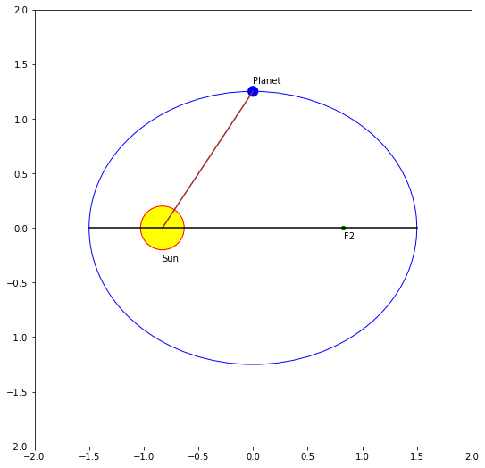
The geometry of the movement of the celestial bodies have been quite well understood since Kepler formulated his well known laws back in the 17th century. They state the planets move around the sun following an elliptical trajectory, with the sun sitting at one of the ellipse foci. In the next figure, we see an (exagerated) elliptical orbit, with its two foci marked as “Sun” and “F2”. An hypothetical planet is also shown over the orbit line.

In [125]:

import numpy as np
from numpy import linalg as la
from matplotlib import pyplot as pl
from matplotlib.patches import Ellipse
from matplotlib.text import Annotation
%matplotlib inline
fig_size = np.zeros(2)
fig_size[0]=12
fig_size[1]=9
pl.rcParams["figure.figsize"] = fig_size

In reality, the planetary orbits are much less eliptical and much more circular. The difference between both axes of the ellipse is very small, so if we drew this to scale, it would resemble a circle. Excepting for Pluto and for Mercury, whose orbits are more elliptical than the rest of planets (please, let’s don’t get started about Pluto).

In [126]:

ax = pl.gca()
semix = 3/2
semiy = 2.5/2
foc = np.sqrt(semix**2 - semiy**2)
ax.set_xlim(-2,2)
ax.set_ylim(-2,2)
elipse = Ellipse(xy=(0,0),width=semix*2,height=semiy*2,ec='b',fc='none')
line = pl.Line2D((-semix,semix),(0,0),color='black')
f1 = pl.Circle(radius=0.2,xy=(-foc,0),fc='yellow',ec='red')
f2 = pl.Circle(radius=0.02,xy=(foc,0),fc='green')
tf1 = Annotation("Sun", xy=(-foc,-0.3))
tf2 = Annotation("F2", xy=(foc,-0.1))
planet = pl.Circle(radius=0.05,xy=(0,semiy),fc='blue')
tplanet = Annotation("Planet",xy=(0,semiy+0.07))
pl.axes().set_aspect('equal')
lrad = pl.Line2D((-foc,0),(0,semiy),color='brown',label="Planet radius")
ax.add_patch(elipse)
ax.add_artist(f1)
ax.add_artist(tf1)
ax.add_artist(f2)
ax.add_artist(tf2)
ax.add_artist(planet)
ax.add_artist(tplanet)
ax.add_artist(lrad)
ax.add_artist(line)

Out[126]:

<matplotlib.lines.Line2D at 0x11f6c2eb8>

Kepler also formulated two more laws depicting the planetary movement and comparing the orbits of the different planets. We can ignore those two laws for the sake of the discussion in this article. Of course you can read the full description in the wikipedia if you are interested.

---

Some people finds counter-intuitive that the planets follow elliptical orbits with just one object in one focus. Some of these people are really vocal saying Kepler was wrong (or even that Kepler didn’t understand his own laws). What we are going to do is to trace the trajectory of an object subject to a gravitational field, and look if it traces an ellipse.

---

How to compute an orbit

Mathematical base

We could try to determine the curve followed by an object using pure calculus. We could part from Newton’s universal gravitation equation: F=Gm1m2r2F=Gm1m2r2

In this formula, m1m1 and m2m2 are the masses of two bodies whose gravitational force we are computing and rr is the distance between them. GG is the Universal gravitational constant, whose value is 6.67384e−116.67384e−11.

That formula gives us the strength of the gravitational force. The direction is always between the two bodies. We can compute the vector of the force that the mass m1m1 exerts over m2m2 using a little bit of vector arithmetics. If you can’t follow it, just don’t worry and enjoy the ride. F→=−Fr→r=−Gm1m2r2r→r=−Gr→m1m2r3F→=−Fr→r=−Gm1m2r2r→r=−Gr→m1m2r3

Now, we know that the acceleration for a body of mas m1m1 subject to a force F→F→ is a=F→m1a=F→m1

We also know the acceleration is the second derivative of the position respect to time, so: d2r→dt2=F→m1=−Gr→m2r3d2r→dt2=F→m1=−Gr→m2r3

Now this is a second order differential equation, that we could try to solve. It would yield r→r→ as a function of t, so we could easily determine which kind of curve our body would follow. We would need to know two initial conditions (one for each integration of the second order equation), which correspond to the initial position and speed of the body.

Easy, uh?

Not so fast!

The n-body problem

I have to confess I cheated. Big time. Because the differential equation I wrote just considers one moving object. In reality, both objects would exert force one against the other, so both would move. So we would have to combine the movements in a bigger equation. And that’s just for two bodies. Imagine three, four… n bodies. Each one pulling every other.

The resulting equation just can’t be solved.

Please understand I’m not saying we don’t know how to solve it. It’s a stronger negative: it can be proved there is no analytical solution for the so called n-body problem. To be more specific:

• The 2-body problem can be solved analytically.
• The 3-body problem can’t be solved in general, but there are some specific solutions for very specific initial conditions; those solutions yield, between other things, the known Lagrange Point orbits.
• For n>3n>3 there are some partial solutions, but it has been proved there is no general solution

---

For our Kepler skeptic the 2-body problem should be enough. The analytical solution shows the orbits are conical sections: elipses, parabolas or hyperbolas, depending on the initial conditions. For the speeds and positions of the planets of our solar system, it yields ellipses with very low eccentricity (thus very close to being circles).

---

But, wait a moment… our solar system is actually a n-body problem. So our two body solutions are just approximations. In reality, we can’t prove our solar system will be stable forever. But this is a digression, and we know it WILL be stable for the duration of our biosphere.

No calculus, please

Solving a second order differential equation is not easy, and it’s beyond the reach of most of mortals. Is there a way to compute orbits without using that calculus witchcraft? Indeed it is. And actually it is quite simple. First we will define a simplified version of our problem, and then we will devise a way to attack it using simple(r) mathematics.

The 1-body problem

It looks like nonsense. To have gravitational attraction, we need at least two bodies. So talking about an “1 body” problem seems a contradiction.

What we will do is to consider the case when one of the two bodies has an insignificant mass in comparison to the other one. For instance, an artificial satellite versus the planet Earth. Or a small moon versus the Sun. The question is if the object has a very small mass, the force it exerts ovet the major body is practically zero. So the other body does not experiment movement due to the accelerarion of its companion.

This allow us to consider the major body as fixed, and conveniently situated at our origin of coordinates (0,0). We can limit our calculations to the moving body, which we will consider has an unitary mass (1 kilogram). So we can write out its mass from the equations, and we have: F→=−Gr→mr3F→=−Gr→mr3

Since the mass of the moving object is 11, then the acceleration it is subject to is just the same A→=F→A→=F→ (with the correct units, of course).

How can we use this knowledge to trace the object orbit? Easy: using the old divide and conquer principle.

Numeric computation of an orbit

We part from known initial conditions: position and velocity. What we will do is really simple: we will compute the gravitational force exerted over our object and then, using a small enough interval of time, we will update our velocity using the acceleration we just computed, and then the position. We will repeat this all the times we want. And we will get a collection of points where our object has aproximately passed.

Our aproximation consists on substituting the real curve by small straight lines. If the lines are small enough, they will approximate the real curve.

Now, let’s do some coding!

In [127]:

# Universal gravitation constant
G = 6.67384e-11


# Gravitational force (vectorial)
def gravity(mass, pos):
    """
    Computes the gravitational force exerted by a body of a specific mass
    located at the coordinate origin against an unit mass located at a
    specific position. The coordinates are assumed to be 2D.
    
    Args:
        mass: The mass of the object located at the coordinate origin (0,0)
        pos: 2D vector containing the coordinates (x,y) of an object of
             unit mass (1kg), in meters
             
    Returns:
        2D vector with the (x,y) components of the gravitational force
    """
    distance = la.norm(pos);        # Compute the modulus of the position
    force = -1.0 * G * mass / distance**2 # Compute the force modulus
    grav = np.multiply(force, pos) / distance   # Compute the gravity force vector
    return grav

This function computes the gravitational force as a vector. In python we will represent our vector as a tuple. To simplify our model we will ignore the third dimension; our object moves thru a plane. Actually, this function would work as well for 3D vectors.

The next two functions compute the updated velocity and position, given a specific time interval.

In [128]:

def velocity(vInit, accel, time):
    """
    Computes the velocity acquired after an acceleration has been applied
    during an interval of time.
    
    Args:
        vInit: initial velocity (vector, meters / seconds)
        accel: acceleration (vector, meters / seconds**2)
        time: Elapsed time in seconds
        
    Returns:
        Vector with the new velocity
    """
    v = vInit + np.multiply(accel,time)
    return v

def position(rInit, velocity, time):
    """
    Computes the position of an object after moving at a specific velocity
    for a specific time.
    
    Args:
        rInit: initial position (vector, meters)
        velocity: velocity of the object (vector meters/secons)
        time: elapsed time in seconds
    Returns:
        Vector with the new position
    """
    r = rInit + np.multiply(velocity,time)
    return r

Finally, we define a function to iterate the object position and give us an array with the computed points which form its orbit.

In [129]:

def orbit(mass, initialPos, initialVel, time, steps):
    """
    Computes the orbital positions of an object of unitary mass (1kg), 
    which specific initial position and velocity, subject to the gravitational
    atraction of another body.
    
    This function computes the positions using a one body setup. That is,
    the big object is considered fixed. The mass of the fixed object has to be
    very big to keep the position error capped.
    
    Args:
        mass: mass of the big, fixed object
        initialPos: initial position of the moving object (vector, meters)
        initialVel: initial velocity of the moving object (vector, m/s)
        time: total calculation time (in seconds)
        steps: number of intervals the time will be divided into
    Returns:
        Array of vectors containing the computed position for each interval
    """
    points = np.zeros((steps-1,2))    # Allocate output array
    pos = initialPos
    v = initialVel
    interval = time / steps
    for i in range(0,steps-1):
        f = gravity(mass, pos)      # Gravity force
        v = velocity(v,f,interval)  # For unitary mass, a = f/1 = f
        pos = position(pos, v, interval)
        points[i,0] = pos[0]
        points[i,1] = pos[1]
    return points

Now we have all the tools we need to plot orbits. We will try to plot the orbit of an artificial satellite. The initial conditions are similar to the ones for the Hubble Space Telescope. Let’s compute its orbit and plot it.

In [130]:

# Earth mass (kilograms)
EM = 5.98000e24

# Earth radius (Metres)
ER = 6371000.0

STEPS = 150         # Number of steps we want to compute
TIME = 97.0 * 60;     # Orbital period in seconds

Altitude = 539000.0    # Altitude of the HST
Speed    = 7600.0      # Approximate speed of the HST
Distance = ER + Altitude


hubble = orbit(EM, (Distance,0.), (0.,Speed), TIME, STEPS)

ax = pl.gca()
ax.set_xlim(-1.25*Distance, 1.25*Distance)
ax.set_ylim(-1.25*Distance, 1.25*Distance)

ax.plot(hubble[:,0], hubble[:,1])
pl.axes().set_aspect('equal','datalim')
earth = pl.Circle((0,0), ER, color='blue')
ax.add_artist(earth)
pl.show()

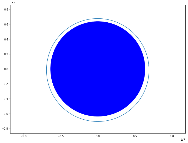
The solid blue circle represents the Earth at approximate scale. As we can see, out quasi-HST traces an almost perfect circle.

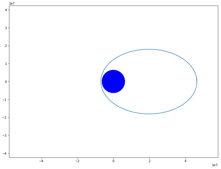
What about an ellipse. Let’s try a Molniya-like orbit. This orbit was discovered by the soviets and is used for communication satellites serving high latitude areas. Our interest is in its clearlu elliptical shape.

In [131]:

Altitude = 40000000.0    # Altitude of the HST
Speed    = 1500.0      # Approximate speed of the HST
Distance = ER + Altitude

STEPS = 500        # Number of steps we want to compute
TIME = 12.5 * 60 * 60;     # Orbital period in seconds



molniya = orbit(EM, (Distance,0.), (0.,Speed), TIME, STEPS)

ax = pl.gca()
ax.set_xlim(-1.25*Distance, 1.25*Distance)
ax.set_ylim(-1.25*Distance, 1.25*Distance)

ax.plot(molniya[:,0], molniya[:,1])
pl.axes().set_aspect('equal','datalim')
earth = pl.Circle((0,0), ER, color='blue')
ax.add_artist(earth)
pl.show()

Conclusion

This plot shows clearly a single mass positioned at one focus generates an elliptical trajectory. The code used to generate the plot is clear and has no hidden catch.

It’s quite trivial to enhance this code to solve a two, three or n body problem. The number of calculations grows very fast with the number of objects, so unless you have access to a supercomputer you should not go very far.

License

This work is licensed under a Creative Commons Attribution-NonCommercial 4.0 International License.

---